This blog will explain the inner workings of gradient descent with an example.

Description

Objects that are thrown up, try to come down; water kept at a height, tries to reach the lowest inclination. These everyday phenomena are common ways through which objects try to obtain stability (lower the height, higher the stability). Built along these lines, we have a famous mathematical algorithm called Gradient Descent – that is used in all sorts of neural networks and machine learning problems.

This blog would help you understand the working of the algorithm and give you an intuition of the same by taking our own life as an example. Machine Learning: A Field of study that gives computers the ability to learn without being explicitly programmed – Arthur Samuel (1959). We can categorize a machine learning problem into 2 categories.

Types of machine learning problems:

1. Supervised Learning
2. Unsupervised learning

Supervised learning

It is a machine learning approach that’s defined by its use of labeled datasets. All the inputs in the dataset are mapped to their corresponding output. Intuitively, the dataset can be considered as your textbook with all the questions (inputs) with their appropriate (answers).

Example

1. Predict Gender based on Name, given a dataset that maps as follows, names-> gender.
2. Predict house rent based on historical dataset that has all house prices.

UnSupervised learning

It uses machine learning algorithms to analyze and cluster un -labeled data sets. These algorithms discover hidden patterns in data without the need for human intervention (hence, they are “unsupervised”). The clustering algorithm is one of the famous algorithms under this set.

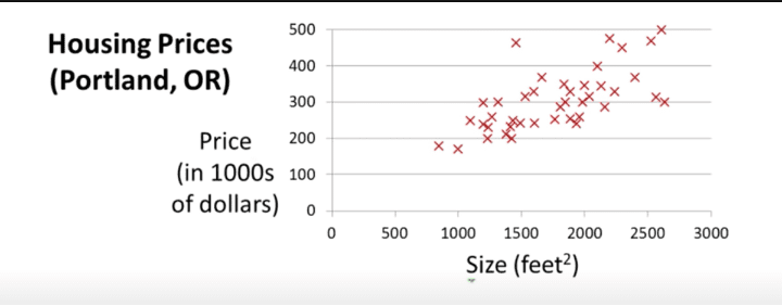
For example, let’s analyse this problem statement, and in the process of solving this problem learn the underlying working principle of gradient descent. We are given a dataset that consists of prices of houses($), the size of the house (feet^2). By using this dataset, we are to build a basic machine-learning model that can predict the price of the house, given the size. There are many ways to solve this problem but let us start with the simplest – Linear regression approach.

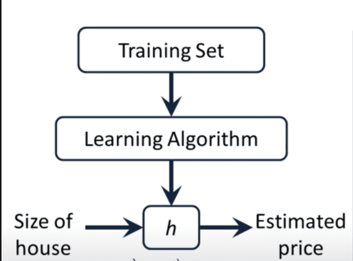
As shown in the above image, we make use of the training set and create a hypothesis. This hypothesis is nothing but a function that gives out the predicted price, given the size of the house.
Input = size of house -> hypothesize -> output = estimated prize.
Now to describe this hypothesis,
y = mx + c;
Sounds familiar? This is the famous equation for a straight line, tweaking the values of m and c it creates all possible straight lines in a 2d plane. Now, we proceed to find the values for ‘m’ and ‘c’, such that our predictions are not far away from the actual value.

Cost Function

The cost function determines how well our hypothesis performs on predicting the price of houses. Higher the value returned by the cost function, indicates a model that is not performing well, and lower the value, indicates a good fitting model.

Our Motive

Choose values of ‘m’ and ‘c’ such that:  h(x) is close to y for our training examples (x,y).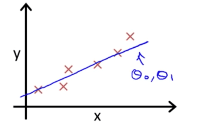

Our goal

Minimize  ∑ ( h(x) – y) ^ 2 for all data points. This is our cost function, that finds the square of the difference between the actual value (y in dataset), and the value predicted by hypothesis (h(x)). Our goal is to minimize the cost function and that in turn would give us a hypothesis

cost function J(m, c) = 1/2n * ∑ ((m*x + c) – y ) ^2;

Where ’n’ denotes the number of items in the dataset.

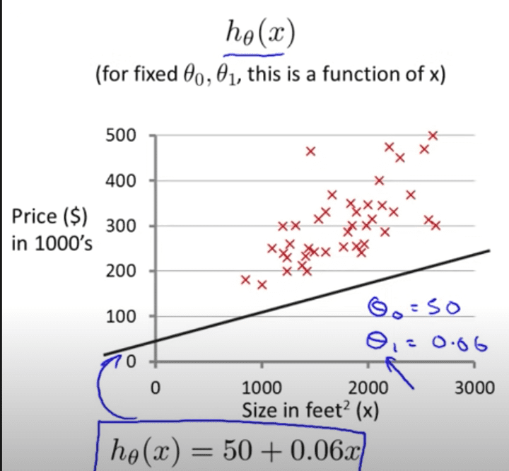
This cost function is called the meansquared error function. Different values of ‘m’ and ‘c’ will generate different straight lines, and each of those straight lines would have different values for the cost function. The one that generates the minimum value for the cost function, we would use those values of ‘m’ and ‘c’ in our hypothesis.

Gradient Descent

It is an iterative first-order optimization algorithm used to find a local minimum/maximum of a given function. This method is commonly used in Machine Learning (ML) and Deep Learning (DL) to minimize a cost/loss function (e.g. in a linear regression).

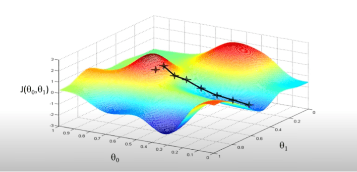
A graph plotted for various values of θ_{0 &} θ_1: against Cost function J, would result in something like this.

Gradient

Before jumping into code, one more thing has to be explained — What is a gradient? Intuitively, it is a slope of a curve at a given point in a specified direction. Because we are interested only in a slope along one axis and ignore the others, these derivatives are called partial derivatives.

Gradient simply put, would tell us about the slope of the function at a given point. Positive value indicates a positive slope and a negative value, a negative slope.

The idea of gradient descent in linear regression is to initialise the value of   θ_{0 &} θ₁  and at each iteration, compute the gradient (slope)and based on the slope, tweak the parameters, this will help us in reaching the local minima for our cost function – which is the best fit in our Linear Regression approach.

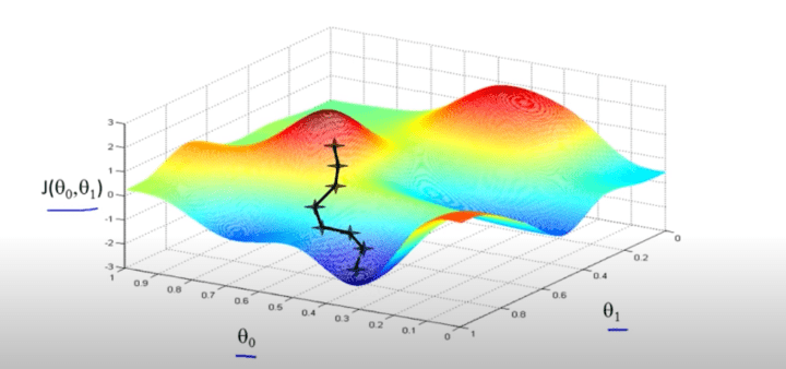
Lowering the value of J (cost function) means, better the modal. Caution even a slight change in the initialisation value might take us to a completely different local minima.

Pseudo code: (Iterating the dataset once is called an epoch)

for i in range(0, iterations):

for j in range(0,2):

θ_j =  θ_j  – ⍶ * slope ;

⍶ : denotes the learning rate.
𝛅/𝛅θ_j (J( θ_{0 ,}θ₁)): denotes the slope of the cost function with respect to a particular variable.(partial derivative).

Simultaneous update of both the parameters, result in quick convergence of the cost function.

Gradient Descent Intuition

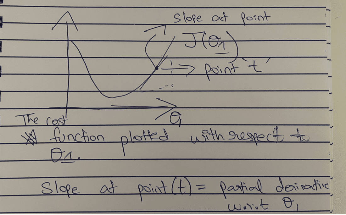
Since our goal is to reduce the value of the cost function, gradient descent should indicate that from point ’t’ we should reduce the value of _,θ_1. As per the graph, we reduce the cost function.

θ₁ =  θ₁  – ⍶(𝛅/𝛅θ_j (J( θ_{0 ,}θ₁)));

(𝛅/𝛅θ_j (J( θ_{0 ,}θ₁))) -> would return a positive value at ’t’ because the slope is positive and upwards.

& learning rate is always ⍶ is always positive number.

Therefore, θ₁ =  θ₁  – ⍶ (+ve number);

Value of θ₁ would obviously reduce, this in turn as per the graph, would reduce the cost function. Partial Gradient of the cost function can be easily found using basic derivatives knowledge.

This Gradient descent algorithm is so powerful that it powers most of the deep learning models for finding the correct hypothesis. With this basic information, you can build a simple linear regression model that predict prices given a dataset.

Now our life is like the gradient descent algorithm, all of us are initialised randomly, some are initialised with advantages( born with a golden spoon) others are not that lucky, but at every step in our life, we try to reach the local minima (better version of our self), and it is our actions – positive or negative, that would determine whether we reach a global optima (best version of ourself) or local optima (average).