Solving the Multi-Camera Puzzle: How Audio Fingerprinting Revolutionized My Video Synchronization Workflow

The Symphony of Chaos: When Multiple Cameras Create a Puzzle

Have you ever worked on a multi-camera production? If so, you’re familiar with the headache: dozens or even hundreds of video clips from different angles, all capturing the same event but with no easy way to determine which clips belong together or exactly where they fit in the timeline.

This was precisely the problem I faced in my project. We had footage from multiple camera angles that needed to be:

• Accurately synchronized to the exact frame,
• Mapped to specific moments in the main footage, and
• Clustered by scene—identifying which clips showed the same moment from different angles.

Traditional approaches were problematic:

• Manual synchronization was painstakingly slow and error-prone.
• Visual feature matching was computationally expensive and unreliable across different angles.
• Timecode-based methods failed because the cameras weren’t professionally synced.

I needed a better solution—one that was accurate, efficient, and scalable.

The Lightbulb Moment: Audio as the Common Thread

While staring at a grid of video thumbnails, I had a realization that would change everything: regardless of camera position or angle, the audio remained relatively consistent across all clips of the same moment. The crowd reactions, dialogue, and ambient noise all formed a unique audio signature, no matter which camera captured them.

This insight led me to explore audio fingerprinting—the same technology that powers apps like Shazam. If my phone could identify songs in noisy environments, could this technology identify matching segments across different video clips?

To gain a deeper understanding of the fundamental workings of audio fingerprinting, take a look at the previous blog that explores the technical foundations of this intriguing technology:

The Invisible Signatures All Around Us: Inside the Magic of Audio Fingerprinting

 Implementing the Solution: A Technical Breakdown

Step 1: Creating the Master Fingerprint Database

The first challenge was breaking down our main footage into a searchable database of audio fingerprints. This proved to be far more complex than it might initially seem.

Traditional audio fingerprinting systems like Shazam are designed to identify complete songs from a database of millions. Our task was different: we needed to pinpoint exact segments within a single continuous recording and match them with short clips from various cameras.

Here’s how I approached creating this specialized fingerprint database:

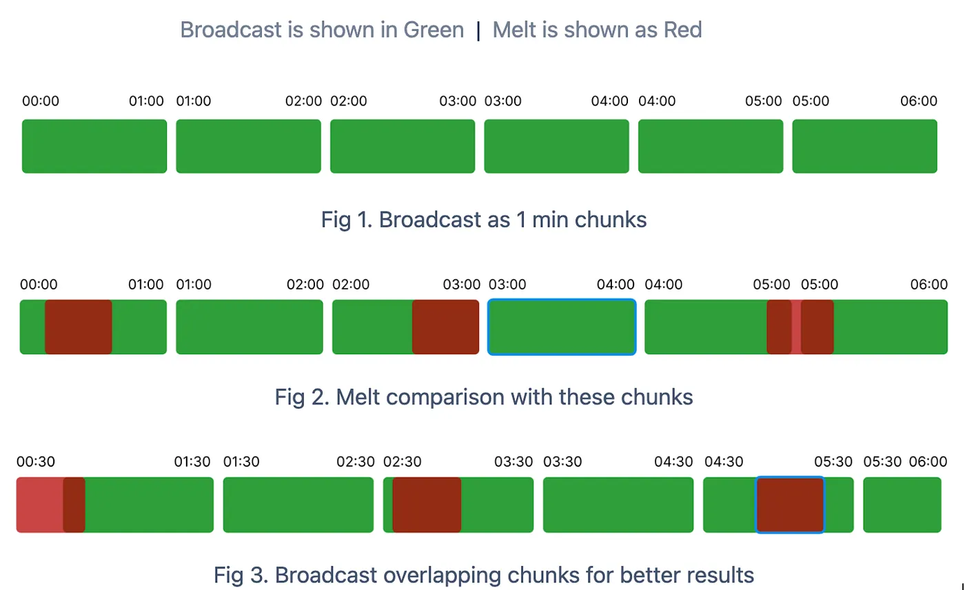
1. Time-Based Chunking: Instead of processing the entire multi-hour recording as a single unit, I divided it into manageable one-minute chunks.
2. Strategic Overlapping: The most critical insight was implementing a 30-second overlap between adjacent chunks. Without this overlap, clips starting near a chunk boundary risked not finding matches. This overlapping approach created redundancy that dramatically improved matching accuracy.

      3. Parallel Processing: To handle the computational demands efficiently, the system processed multiple                       chunks simultaneously using Python’s concurrent processing capabilities.

Here’s the code that powers the carefully crafted chunking and fingerprint-database creation process.

def split_audio_track_to_chunks(self, audio_file_path, interval_ms=60000):
    # Load the audio file
    audio = AudioSegment.from_file(os.path.join(self.root_dir, audio_file_path))
    
    # Get the length of the audio in milliseconds
    audio_length_ms = len(audio)
    fingerprint_data = []
    
    # Process chunks in parallel for efficiency
    with concurrent.futures.ThreadPoolExecutor() as executor:
        # Create both standard and overlapping chunks to ensure better matching
        for i in range(0, audio_length_ms, interval_ms):
            # Standard chunk
            end_time = min(i + interval_ms, audio_length_ms)
            start_timestamp = self.ms_to_hms(i)
            end_timestamp = self.ms_to_hms(end_time)
            chunk = audio[i:end_time]
            future = executor.submit(self.get_fingerprint_data, chunk,
                                     start_timestamp, end_timestamp)
            futures.append(future)
            
            # Create overlapping chunks for better matching at boundaries
            overlap_start = i + 30000  # 30-second overlap
            overlap_end = min(end_time + 30000, audio_length_ms)
            if overlap_start < audio_length_ms:
                overlap_start_timestamp = self.ms_to_hms(overlap_start)
                overlap_end_timestamp = self.ms_to_hms(overlap_end)
                chunk = audio[overlap_start:overlap_end]
                future = executor.submit(self.get_fingerprint_data, chunk,
                                         overlap_start_timestamp,
                                         overlap_end_timestamp)
                futures.append(future)

The  get_fingerprint_data() method was responsible for generating fingerprints by leveraging the capabilities of acoustID.

def get_fingerprint_data(self, chunk: pydub.AudioSegment, start, end):
    if not self.is_silent_track(chunk):
        audio_segment = chunk

        audio_data = audio_segment.raw_data
        audio_data = self.convert_audio_to_buffer(audio_data)

        # Generate and encode the fingerprint in one step

        try:
            fingerprint = acoustid.fingerprint(audio_segment.frame_rate, audio_segment.channels,
                                               audio_data)
            fingerprint, _ = acoustid.chromaprint.decode_fingerprint(fingerprint)

            result = {
                f'{start}_{end}': {
                    'start_timestamp': start,
                    'end_timestamp': end,
                    'fingerprint': fingerprint
                }}
            return result
        except TypeError as e:
            print(f"Error decoding fingerprint: {start}_{end}: {e}")
            return {}
    else:
        return {}

The key optimization was creating overlapping chunks. This ensured that even if a clip started in the middle of a reference segment, we would still find a match.

Step 2: The Magic of Matching

With fingerprints generated for both the main footage ‘s fingerprint database and the individual short clips, the next challenge was matching them accurately and determining the exact timestamp positions. This was the heart of the entire system.

Here’s how the matching algorithm worked:

def search_matches(broadcast_audio, melt_audio):
    fp_full = broadcast_audio  # Fingerprint from database chunk
    fp_frag = melt_audio       # Fingerprint from short clip
    
    # Convert fingerprints to 20-bit format for more efficient comparison
    full_20bit = [x & (1 << 20 - 1) for x in fp_full]
    short_20bit = [x & (1 << 20 - 1) for x in fp_frag]
    
    # Find common fingerprint elements
    common = set(full_20bit) & set(short_20bit)
    
    # Create inverted indices for faster lookup
    i_full_20bit = invert(full_20bit)   # Maps each fingerprint value to its positions
    i_short_20bit = invert(short_20bit)
    
    # Count offsets between matching fingerprint points
    offsets = {}
    for a in common:
        for i in i_full_20bit[a]:
            for j in i_short_20bit[a]:
                o = i - j  # This offset represents potential alignment points
                offsets[o] = offsets.get(o, 0) + 1
    
    # Find the strongest potential matches based on offset clusters
    matches = []
    for count, offset in sorted([(v, k) for k, v in offsets.items()], reverse=True)[:20]:
        # Calculate bit error rate (BER) to assess match quality
        matches.append((ber(offset), offset))
    matches.sort(reverse=True)
    
    return fp_frag, matches

The core insight of this matching algorithm was focusing on the relative positions of fingerprint features rather than simply comparing raw fingerprints. This approach, inspired by Shazam’s landmark-based algorithm, proved remarkably resilient to background noise and variations in audio quality.

Once a match was found, the next critical step was translating the fingerprint offset into an actual timestamp position:

def get_matching_timeframe(fp_frag, matches, broadcast_fragment_start_timestamp):
    if matches:
        score, offset = matches[0]
        
        # Convert fingerprint offset to actual seconds
        offset_secs = int(offset * 0.1238)  # each fingerprint item represents 0.1238 seconds
        fp_duration = (len(fp_frag) * 0.1238 + 2.6476)  # empirically determined duration
        
        end_secs = offset_secs + fp_duration
        hours, minutes, seconds = map(int, broadcast_fragment_start_timestamp.split('-'))
        broadcast_start_time = timedelta(hours=hours, minutes=minutes, seconds=seconds)
        actual_start_time = broadcast_start_time + timedelta(seconds=offset_secs)
        actual_end_time = broadcast_start_time + timedelta(seconds=end_secs)
        
        actual_start_time_str = AudioFingerprintUtils.timedelta_to_str(actual_start_time)
        actual_end_time_str = AudioFingerprintUtils.timedelta_to_str(actual_end_time)
        
        return score, actual_start_time_str, actual_end_time_str

Step 3: Connecting the Dots Between Cameras

Beyond just mapping clips to the timeline, I needed to identify which clips showed the same scene from different angles. This required a clever approach to implement fingerprint similarity:

def cluster_melts(fingerprint_dict, scene_matrix):
    # Generate all possible pairs of fingerprints for comparison
    fingerprint_pairs = [([0, fingerprint_dict[f1]], [0, fingerprint_dict[f2]])
                         for f1, f2 in combinations(fingerprint_dict.keys(), 2)]
    file_pairs = [(f1, f2)
                  for f1, f2 in combinations(fingerprint_dict.keys(), 2)]
    
    # Parallelize fingerprint comparisons for efficiency
    with concurrent.futures.ProcessPoolExecutor(max_workers=num_processes) as executor:
        similarity_scores = list(executor.map(compare_fingerprints, fingerprint_pairs))
    
    # Create a DataFrame to store comparison results
    scenes_comparison_results = pd.DataFrame({
        'scene': [pair[0] for pair in file_pairs],
        'compared_scene': [pair[1] for pair in file_pairs],
        'similarity_score': similarity_scores
    })
    
    # Filter to keep only meaningful similarities (above threshold)
    scenes_comparison_results = scenes_comparison_results[scenes_comparison_results['similarity_score'] > 0.5]
    
    # Build a graph and identify clusters of similar clips
    G, groups = group_similar_audio_files(scenes_comparison_results)
    
    # Assign event/group labels to the scene matrix
    for event_no, files in groups.items():
        scene_matrix.loc[scene_matrix['scene_no'].isin(files), 'event'] = event_no
    
    return scenes_comparison_results

Like a detective connecting evidence on a corkboard with red string, the core logic meticulously filtered through thousands of potential clip relationships. The system only selected the strongest connections, those with similarity scores that exceeded the critical threshold. Then, using connected components analysis, the system grouped these individual relationships into coherent clusters, showing which camera angles were related even if their direct links were difficult to find.

def group_similar_audio_files(df, similarity_threshold=0.5):
    # Create a graph
    G = nx.Graph()
    
    # Add edges for pairs above the similarity threshold
    for _, row in df.iterrows():
        if row['similarity_score'] >= similarity_threshold:
            G.add_edge(row['scene'], row['compared_scene'], weight=row['similarity_score'])
    
    # Find connected components (clusters)
    clusters = list(nx.connected_components(G))
    
    # Create a dictionary to store the groupings
    groupings = {}
    for i, cluster in enumerate(clusters):
        groupings[f"Event_{i + 1}"] = [int(x) for x in cluster]
    
    return G, groupings

This graph-based approach had several advantages:

1. It naturally handled transitive relationships—if clip A was similar to clip B, and B was similar to clip C, all three would be grouped together even if A and C had lower direct similarity.
2. It provided visual representations—the system generated network graphs visualizing the relationships between clips, making it easy to spot clusters at a glance.
3. It created logical “events”—each connected component in the graph represented a distinct moment captured from multiple angles.

 

The system also included a recursive mapping approach for clips that couldn’t be directly matched to the timeline but could be matched to other clips that were already mapped. This “mapping by association” approach dramatically increased the system’s overall success rate, allowing us to place clips even when their direct audio match was too weak or noisy to be reliable. If clip A couldn’t be directly matched to the timeline but was visually identical to clip B, which had been successfully matched, we could confidently place clip A at the same timeline position.

The Results: Transforming Our Workflow

The impact of this audio fingerprinting approach was dramatic:

1. Accuracy Beyond Expectations

The system achieved sub-second alignment accuracy—often identifying the exact frame where clips belonged in the timeline. This level of precision would have been impossible to achieve manually.

2. Dramatic Time Savings

What previously took several days of manual work was now accomplished in minutes. For a project with hundreds of clips, this reduced weeks of synchronization work to a single overnight processing run.

3. Discovery of Hidden Connections

The fingerprint similarity clustering revealed relationships between clips that were not visually obvious. In several cases, we found usable alternate angles for key moments that we might have otherwise missed.

Technical Challenges and Solutions

Challenge 1: Processing Efficiency

With hundreds of audio segments to fingerprint and compare, computational efficiency became critical. The solution was aggressive parallelization: By utilizing  ProcessPoolExecutor  with careful consideration of CPU core counts, the system could process hundreds of fingerprints simultaneously.

Challenge 2: Silent or Music-Only Segments

Some clips contained no distinguishable audio or only background music, making fingerprinting difficult. To address this, I implemented a pre-filtering step:

@staticmethod
def is_silent_track(audio_segment, energy_threshold=-60):
    """
    Checks if an audio segment is silent by analyzing its audio energy.
    Returns True if the audio segment is silent, False otherwise.
    """
    # Calculate the audio energy in dBFS (decibels relative to full scale)
    audio_energy = audio_segment.dBFS
    # Check if the audio energy is below the threshold
    return audio_energy < energy_threshold

This allowed the system to skip silent segments and focus processing resources on clips with usable audio content.

Challenge 3: Handling Unmapped Clips

Not all clips could be directly matched through audio fingerprinting. For these, I developed a recursive matching approach that leveraged already mapped clips:

This “mapping by association” method allowed the system to handle clips where direct audio fingerprinting failed but a similarity to another clip could be established.

Broader Applications: Beyond My Project

This audio fingerprinting approach has implications far beyond my specific use case:

1. Live Event Multi-Camera Production: Synchronizing footage from multiple cameras at concerts, sports events, or conferences.
2. User-Generated Content Aggregation: Organizing clips from the same event uploaded by different users.
3. Documentary Filmmaking: Aligning historical footage from various sources.
4. Security Camera Analysis: Synchronizing footage from multiple security cameras.

Lessons Learned and Technical Insights

Throughout this project, several key insights emerged:

1. Audio > Video for Synchronization

While visual cues might seem like the obvious choice for video work, audio has proven to be far more reliable and computationally efficient for synchronization purposes.

2. Preprocessing is Critical

The quality of fingerprinting results depended heavily on preprocessing steps such as silence removal and normalization. The time invested in these steps yielded huge dividends in matching accuracy.

3. Parallelization is Non-Negotiable

For any production-scale implementation, aggressive parallelization is essential, as both fingerprint generation and matching benefit from multi-core processing.

Conclusion: The Future of Audio-Driven Video Workflows

Audio fingerprinting has fundamentally changed how I approach multi-camera production workflow. What began as an experiment has become an indispensable part of our production pipeline.

As media production continues to involve more cameras and sources, techniques like this will only become more valuable. The ability to automatically organize and synchronize footage without relying on professional timecode systems opens up possibilities for productions at all budget levels.

The next frontier? The next frontier pushes us to adapt this technique for tougher audio conditions and leverage machine learning to further improve fingerprinting accuracy. Realizing that every video’s soundtrack contains a hidden key to unlocking powerful automation opens up endless possibilities.